 |
MULTIPLE CHOICE TESTS Processing Test Marks by Eric Scharf |
 |
| MCQ? Options Raw Data Average Max Penalty Evaluation Subtract Future Conclude Refs Date Read Me |
Abstract
| This "web-paper" presents the mathematical basis for the processing of the marks for examinations comprising multiple-choice questions, where the examinations lead to actual qualifications. Whilst the gathering of the raw marks produced by multiple-choice tests in self test mode can be automated, it is not always appreciated that the number R of questions a student gets right, as given by the test, is not necessarily the same as the number K of questions for which the student actually knows the answer. To find K, requires a viable model that relates K to R. In this web paper, the implications of using possible schemes for the processing of the raw marks R are examined; it is shown - using simple algebra - that such schemes can differ widely in terms of the final overall mark that a student receives for a multiple-choice test. Without trying to be unduly prescriptive, I would suggest that the averaging marking scheme, using the number of questions actually attempted, together with 3 or 4 choices per question, is likely to be the fairest approach in most educational cases. |
What you will see here
- Introduction, Challenges and Background
- Logistics for this Paper
- Basic Assumptions
- Processing Options
- Raw Data - No Further Processing
- Average or Statistical Approach
- Putting our equations to the test
- Subtraction Approach
- Future Challenges
- Conclusions
- Reference & Links
- Symbols and Abbreviations Appendix
- Finding the Number Q of Questions Attempted
- Spoken Narrative.
This is a quick one-minute audio presentation of this web page. This audio clip should work with the three main browsers, but please click here if you would like more logistical details on this audio presentation.
- Contact, Copyright & "Readme"
Please click here for more general considerations relating to this page and other pages on this web site.
1. Introduction, Challenges and Background
It is helpful to the reader if we say at the outset what a multiple-choice test (MCT) actually is, and indeed, what the advantages and disadvantages are of deploying this kind of test in an educational context. Essentially, we shall start to steer towards the rationale for this "web paper".
1.1 Multiple-Choice Tests
A multiple-choice test (MCT) consists of a series of multiple-choice questions (MCQs). We shall assume in this web paper that each multiple-choice question (MCQ) consists of a number of possible answers or choices, only one of which is actually the right answer.
The following is an example of a typical multiple-choice question.
|
Which one of the four places given below is the capital of Austria?
|
1.2 Uses, Advantages and Challenges of Multiple-Choice Tests
Multiple-choice tests have two main applications, namely: (1) Self learning (auto didactic) and (2) Assessment under examination conditions. For both applications, the speed of marking by the computer can be of tremendous benefit: in the first case it allows almost immediate feedback to the student as regards his or her knowledge of the subject; in the second case, it can also significantly speed up the marking process while making it less error prone compared to a manual approach.
In what follows, we shall refer to the "raw data" which is the immediate output (the results) of a multiple choice test (MCT) before even considering any further processing. Section 5, below, looks in more detail at the relevance of "raw data".
-
Self-Learning. In this mode the student is examining him or herself. Any efforts by the student to reach the correct answer are normally purely concerned with the subject matter in hand, and not coloured in any way by the wish to gain the maximum marks possible. After all, in the self-learning context, the marks gained are purely a personal matter and will not count towards any final official examination marks. Feedback to the student about his or her performance in the MCT can be immediate - either on a per question or on a per test (i.e., a set of questions) basis.
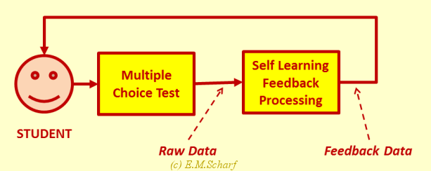
Fig. 1.2.1: MCT in Self-Assessment Mode -
Assessment/Exam Mode. Here the marks of the MCT will count towards the final official marks for a student. There are at least two challenges for the examiners using MCTs for their students. How can a question setter determine:
- if the student actually knows the answer or has produced the right answer by accident for example (1) by guessing or (2) for some other reason such as being distracted?
- the thought processes that lead a student to decide on a particular answer from the choice of available answers?
The second point can to a certain extent be accommodated by a written examination paper, without, of course, the convenience of automated marking which is the advantage of MCTs. In the context of automated marking, the elucidation of a student's thought processes is still very much a research topic - with some results - as references [ref6] to [ref9] at the end of this paper testify.
The first point lends itself to a treatment by the simple maths - often not widely appreciated - which will figure in this paper. Bound up with this there is also a popular way of coercing the student, by a penalty approach, into avoiding incorrect answers; this is also considered in this paper. Penalising a student works against encouraging a student to enjoy the educational experience and should, some may justifiably argue, be kept to a minimum.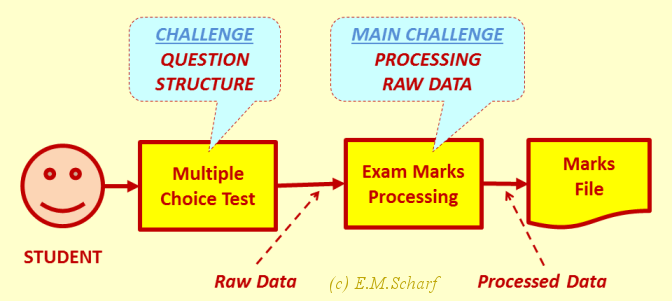
Fig. 1.2.2: MCT in Examination Mode.
Challenge: Why and how should we process the raw data?
Challenge: How many choices for each question? (Question structure).
1.3 Why this paper?
In the humble experience of the author, the implications of using specific processing options for the raw marks from a MCT are not always understood. The nature of the transformation ("black box") between the raw MCT marks and the final official marks for a student is of course crucial. The different types of transformations used can result in a wide variation in the target marks for a student. The author of this paper therefore believes that clarification regarding the possible options is long overdue!
Indeed, the initial experiences of the author, regarding the lack of understanding about multiple-choice tests (MCTs) in the educational sector, led to a paper [ref1] in which the author was the lead contributor. This paper provides an important initial basis for the present web paper.
Further investigations by the author revealed an earlier and seemingly forgotten article [ref3] dating from 1988. This latter paper refers to a "Formula Scoring" method. Unfortunately, the paper [ref3] does not give a clear presentation of the "Formula Scoring" method and the implications of its deployment for multiple-choice tests (MCTs); it is hoped that the present paper can go some way to provide firm mathematical clarification of these issues. Other processing approaches for MCTs include those used by the exams of Australian Mathematics Competition [ref4] which have what appears to be an ad hoc approach to processing the output marks from the MCTs.
Both the author's initial experiences and subsequent investigations led to the present web paper, which, it is hoped, may help to clarify the issues surrounding the processing of the raw marks given by MCTs.
2. Logistics for this Paper
This paper - as mentioned - derives in part from a previous refereed publication [ref1] by the author. This present web paper, however, should be viewed as a living document, whose contents may be amended from time to time to accommodate the latest information. Before checking for the latest update to this web page, don't forget to refresh this page; after that, go straight to the date from here or directly via the "Date" tab at the top of this web page.
In this paper I shall repeat myself in various places with the aim of emphasising and explaining relevant points. In this respect I beg to differ with those academics and others who express a devotion to the hapax legomenon (or ‘απαξ λεγομενον if you wish), for it is by repetition that we learn so many things including the one (or more!) languages that we speak and use in daily life.
I have found that the popular browsers listed in the browser table on the "read me" page display the contents of this page - including the equations - correctly when executing in the machine and operating system environment which is also given on the "read me" page. However, I cannot, of course, guarantee that this will be the case for all browser, machine and operating system environments.
For future reference, if you reached this page by another route, you can also access this page by putting ONE of the following shortcuts in your browser.
3. Basic Assumptions
In the mathematical developments in sections 3 and 4, we shall make the following assumptions, which should not normally affect the generality of the arguments.
- Marks per question. For the purposes of this web paper, each question to which a right answer is given, earns one mark. This should not affect the generality of the derived equations, since, if each right question earns a mark other than one (as long as it is the same mark for each question answered correctly), appropriate scaling can be employed. Of course, in MCTs where questions have different numbers of choices, then we are looking at several smaller or component MCTs, where all the questions in a particular component MCT share the same number A of choices.
- Choices per question. Each one of the questions in a multiple-choice test (MCT) has the same number A of possible choices.
- Right answers per question. Only one of the A possible choices is the right answer. This is the usual practice and we shall not consider the possibility that more than one of the A choices for a question could be right.
- "Rightness" and Knowledge. The student may give a
right answer to a particular question, but that right answer may have been achieved by chance and may therefore not be a statement that the student actually knows the answer.
- Negative Result. If the final mark resulting from applying processing to the raw marks is negative, it is floored to zero, which normally makes practical sense!
Two further points should be made at this juncture.
- Key Equations. For the equations that follow in the next section, dotted red borders indicate key definitions or key derived equations, as appropriate.
- Mathematics is a tool and not an end in itself. The mathematics employed here is of course merely used as a tool or vehicle to put the salient points across to you the reader. The mathematics used here - whether you regard it as simple or complicated - is not of course the end of this presentation in itself! Of course, the simpler the maths, the better. Mathematical simplicity should be seen as a benefit and certainly not as an adverse comment on the intellectual - such as it may be - content of this paper!
4. Processing Options for Multiple-Choice Tests
We now look at three options. They are ways of dealing with wrong ("none right") answers in order to get at the number K of answers that a student actually knows as opposed to the number R of answers a student gets right. Note that the term "wrong" is used to refer to the questions that a student does not get right as opposed to the questions for which a student does not know the answer.
- Raw Data. This option does NO processing at all. (Chapter 5).
- Averaging with questions ATTEMPTED. This option looks only at the questions attempted. It obtains K by subtracting from R a term based on the statistical information about the occurrence of questions whose answers are right by chance. (Chapter 6.1 to 6.3).
- Averaging with questions OFFERED. (Maximum Penalty). This option also includes the questions which have not been attempted. As before, it obtains K by subtracting from R a term based on the statistical information about the occurrence of questions whose answers are right by chance. (Chapter 6.4).
These options are evaluated in chapter 7 further below.
There is also an often "harsher" subtractive approach (chapter 8) which, like the "averaging" approach, can also use either the number of attempted questions or the number of offered questions.
Fig. 4.1: MCT Processing Options.
5. Raw Data - No Further Processing
Here the output marks produced directly by the MCT are regarded as raw data and are not subject to further processing apart from scaling. We could of course assume that the same number (M) of marks (where M is 1 or more) is allocated to each question for a right answer, and scaling is merely a matter of multiplying the number (R) of right questions by M. In the context of our mathematical analysis, it is easiest here to assume, without loss of generality, 1 mark per right question.
Here we repeat for clarity the following distinctions which were alluded to in section 1.2 above.
- Raw Marks. The raw marks (R in number) are produced by the student in response to the student giving the right answers to one or more questions. As mentioned, we assume in this web paper 1 mark per question for a right answer to that question. The raw marks will intrinsically also give the total number Q of questions attempted. The raw marks can also be viewed as the dynamic data for any particular instance of multiple-choice test.
- Structural Data, as the name implies, comprises the static data for a set of questions, namely A, the number of choices per question and, if needed, T, the total number of questions offered.
- Raw Data. Raw data comprises both the dynamic data (R and Q) and the static data (A and, if needed, T) for any particular instance of multiple-choice test.
In this "Raw Data" case, students can gain marks by guessing (i.e., by luck), and, on average, 1/A of the guesses will be correct, where of course we assume that there are A possible choices for a question, only one choice of which is right. This will be so, even if the students have absolutely no knowledge of the actual topic being examined, since wrong results are not penalised.
In other words, this simple approach does not attempt to distinguish between answers resulting from genuine knowledge, and those resulting from lucky guesses. This scenario is usually different from a conventional written paper, where to gain any marks at all, some correct response - written or pictorial - is normally required of the student. In other words, a written paper is more likely to elicit a student's thought processes than a multiple-choice test. The present web paper is a testimony to the fact that I certainly do not give up entirely on the merits of multiple-choice tests, but that, at the same time, I would advocate great caution, for the devil can reside in the detail!
Remember also, in the context of "Raw Marks", that the computer conveniently gathers the marks for us; what we do - or ask the computer to do - with those marks is up to us as the assessors and could have a significant effect on a student's marks in the MCT. This should be a significant message of the subsequent sections of this "web paper".
|
Exam Rubric. When using the "Raw Marks" processing option (i.e., avoiding any subsequent processing), a typical exam rubric could include the following statements. "There is no penalty for a wrong answer. You are therefore urged to attempt every question. If you feel you do not know the answer to a question you should select the answer that you feel is the most likely." |
However, the raw data approach is well suited to self-learning, in other words the auto-didactic context, where the student is examining himself or herself.
6. Average or Statistical Approach
How can we devise an approach that aims to determine the number of questions that a student actually knows as opposed to the number of questions that a student gets right?
We shall develop this theme in the following sections of this chapter.
- Deriving a Formula
- Deriving the Averaging Formula by Another Way
- Using the Averaging Approach
- Averaging with Maximum Penalty
- Averaging with Raw Data
6.1 Deriving a Formula
The total number (R) of questions that a student gets right, is the sum of the number (K) of questions that the student actually knows, plus the number (C) of questions that the student gets right by chance.
| DEFINITION | R = K + C | [1] |
We are after determining the number (K) of questions the answers to which a student knows, and not the number (R) of questions that a student happens to get right and which is what an MCT gives us in the first instance as raw data. In other words, we need to consider:
| K = R − C | [2] |
Of course, to increase our understanding of C, we could ask what causes a student to get by chance the right answers to - possibly - just some of the questions attempted. Put the opposite way, what causes a student to get the wrong answer to any particular question attempted? In this case, for example, a student might:
- take a guess at the questions he or she doesn't know, in the hope of producing a right answer.
- be influenced by the way he or she responded to how the course material being examined was actually taught.
- mistakenly think he or she knows the answer.
- by accident - perhaps by being distracted - put down the wrong answer.
We now consider the general situation, where exam performance is assessed anonymously in order to try to avoid the slightest hint of bias. In this case, the examiner has absolutely no knowledge - not even of the four considerations just considered above - about any particular candidate's reason for getting C questions right by chance. We try to find a plausible model for C.
This can be done by assuming that all questions carry equal weight and that for each question there are "A" possibilities, typically 3 or 4, of which only one possibility is right. In addition, we let Q be the total number of questions attempted. In this case, the number (C) of questions that are right by chance can be obtained by saying that the proportion (1/A) of the (Q-K) questions that a student does not know but has attempted, will - on average - contribute to those questions that appear as being right in the test. This gives:
| DEFINITION |
|
[3] |
Equation [3] is our basic model for relating C to what we wish to find, namely K, the number of questions a student actually knows. While there may be other possible options - such as some weighted least squares formulation of the above four considerations - to determine C, the model in equation [3] is attractively simple, generally applicable and - as we shall see - useable in practice.
We can now use elementary algebra to combine equations [1] and [3] to give us:
|
[4] |
or, rearranging,
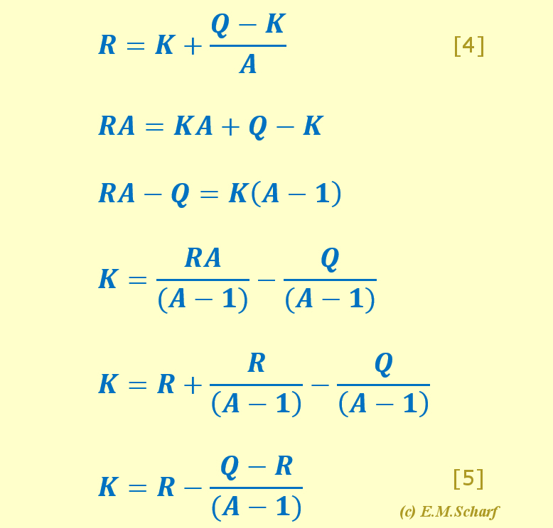
| key derived equation |
|
[5] |
Equation [5] shows that the (Q-R) wrong results will penalise the student. Essentially, in equation [5], in order to obtain K, we reduce the number R of right questions, which the test gives us, by a penalty factor based on the number (Q-R) of wrong answers divided by the number (A-1) of wrong possibilities for each question. Equation [5] thus reflects the fact that the more possibilities (i.e., the higher the number A of choices per question) there are, the more difficult it is to guess correctly the right answer. (Note, as an aside, that in this equation, negative values of K can be forced to a floor value of zero, which is then the minimum mark a student can achieve.)
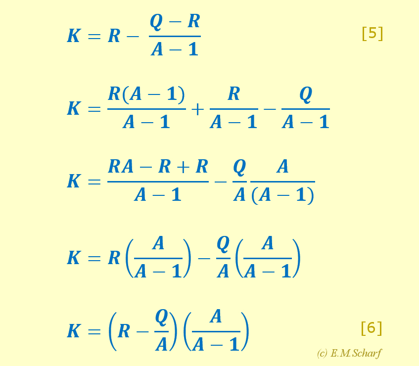
6.2 Deriving the Averaging Formula by Another Way
We shall check our thought processes by using another route to our Averaging Formula, and on the way getting a formula that could be useful for mechanization such as in a spread sheet.
We have said that the zero-penalty option is not ideally suited to an examination context, since it will, on average, give a student Q/A marks - even if that student has no knowledge whatsoever of the exam subject. So, we can subtract this from the number R of "right" answers which the computer has given us. We then need to rescale the resultant number by (A/(A-1)) to get back to our original scale of 1 to Q marks. This gives equation [6] below.
| working equation |
|
[6] |
From the last but one equation [5] above we can, after four algebraic steps, also reach equation [6] just above. Conversely, from equation [6], we can reach equation [5]. This indicates that either approach - via [5] or [6] - gives the same result! We could also relate equation [4] and [6].
![relate equation [4] and [6]](pics/algebra46.PNG)
We can easily "mechanize" the previous equation [6], just above, in a spread sheet.
- For the whole MCQ exam we know "A" and thus we need to pre-calculate only once the terms (1/A) and (A/(A-1)).
- Applying separately to each individual candidate are the variables R and Q. Conveniently R and Q only appear once in equation [6] above for each candidate. R and Q should of course both be expressed in the same units (e.g., typically per 20 or percent). For each candidate only two multiplications (by (1/A) and by (A/(A-1))) will be needed. In an educational context, results will normally be rounded to integers.
In other words, we have the following.
| for WHOLE test: | A: (1/A) and (A/(A-1)), pre-calculated just once | |
| for EACH candidate: | given: R, Q; find K |
In equation [6] we can see that as A tends to infinity, i.e. the number A of choices per question becomes infinitely large, K will tend to R. I'm sure you'll agree that this makes sense! If Q, the number of questions attempted, is replaced by T, the number of questions offered, then we have the "maximum penalty" situation of section 6.4 further down. T, of course, would be valid for every student in the exam; in the "maximum penalty" case, if a student gives no answer for a question that question is treated as being given a wrong answer.
We can also express equation [6] as equation [7] below, which some may prefer for "mechanizing" in (e.g.) a spread sheet.
| alternate working equation |
|
[7] |
6.3 Using the Averaging Approach
|
The Averaging or Statistical Approach requires the number Q of questions attempted by the student, NOT the number T of questions offered to the student. Then the examiner needs to know the number R of questions to which the student has given right answers, either by knowledge or for some other reason. This number R, and the number A of choices per question, will then allow the examiner to find out, on a statistical basis, the number K of questions for which the student actually knows the answer. |
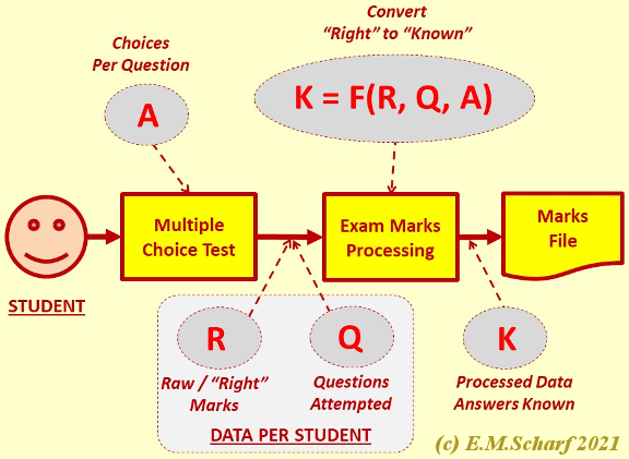
Fig 6.1: Processing using the Averaging Approach with Questions Attempted.
With this averaging or statistical approach, a student attempting a given number X of questions, all of which are answered correctly, may get more marks than his or her colleague who attempts Y questions, where Y > X, but where still only X questions are answered correctly. This is fair because the "Y" student has used up more questions (i.e., more possibilities to get marks). This is illustrated in table in Figure 7.1.1 in section 7.1 below. With the average or statistical approach, it should be emphasized that in any given class examination based on an MCT, each student will have his or her Q value (the number of questions attempted), equal to, or below, the total number of offered questions.
Exam Rubric. When using the Averaging/Statistical processing option, a possible rubric for an examination paper could read as follows. "You will only be assessed on questions which you have attempted. It is recommended that you avoid guessing an answer to a question." (Avoiding guessing is of course highly relevant with the averaging/statistical approach!) |
6.4 Averaging with Maximum Penalty
Here we consider all questions, even those that are not attempted. In other words, questions which are not attempted are assumed to be answered incorrectly - the answers will be regarded as "not right". In this case, we substitute for Q, the total number of questions attempted, the value T, representing the total number of questions offered. In all cases other than the case where the student gets all offered questions right, this variant with T will penalise a student to a greater extent than staying with Q.
Note that with a written paper the usual requirement for obtaining full marks is only to attempt a subset of questions offered. In an MCT full marks can usually only be obtained by answering all questions correctly.
Effectively, with the Maximum Penalty approach, we take equation [5] and replace Q, the total number of questions attempted, by T, the total number of questions actually set. We regard the questions that have not been attempted, as being attempted and wrongly answered - hence the term "maximum penalty". This then gives the following equation, which is the limiting case of equation [5] when all the questions have been attempted. The subscript "AT" refers to the combination of the averaging approach with the consideration of the total number T of questions offered.
|
[8] |
Another form of the Maximum Penalty Equation can be derived, by assuming M marks per question, and putting S = KAT M and SMAX = T M. Here you can see the development from equation [8] to [9]. This gives the following equation:
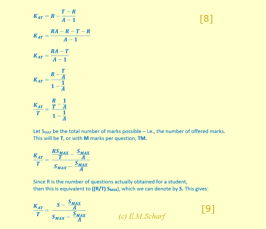
|
[9] |
Equations 8 and 9 are given for completeness, but their presence here should not detract from the main mathematical or algebraic development in this web paper. Hence the symbols used in equations 8 and 9, unless used elsewhere in this paper, on purpose have been excluded from the table of symbols and abbreviations in section 11.
|
Exam Rubric. When using the "Maximum Penalty" approach to processing the results of an MCT, a possible rubric for an examination paper could read as follows. "You will be assessed on ALL questions in this examination, even on those you have not attempted. It is recommended that you avoid guessing an answer to a question." (Of course, a rubric like this could be seen as an invitation to guess!) |
6.5 Averaging with Raw Data
Let us skip back for a moment to our "Raw Data" section 5 and let us at the same time refer to equation [4] in section 6.1. If the student knows absolutely nothing, we can put K=0 in equation [4] in section 6.1. "R" is then the number of "right" questions, which is the result for the MCQ test whose results are based solely on Raw Data. "Q" is the number of questions attempted. In this case, we get:
|
[9A] |
This gives R = (Q/A), as we stated in the "Raw Data" section 5. Thus, if the student knows absolutely nothing regarding the subject matter of the MCQ exam, the student will still, get, on average (Q/A) marks, where Q is the number of questions attempted. Thus, basing the results only on raw data (the "right" results) will, on average, give us an incorrect representation of a student's knowledge of the topics in the MCQ exam. By "incorrect" we mean that the student will on average gain marks even if the student's knowledge of the topics is non-existent! This is not what an exam is intended to do!
The derivation of equation [6] in section 6.2 ("Deriving the Averaging Formula by Another Way"), uses this train of thought in order to modify the number "R" of "right" answers to get to a value for "K", the number of questions the answers to which the student actually knows!
7. Putting our equations to the test
In this section we shall try and "breathe life" into the theoretical results we derived above by seeking answers to the following questions.
- How does the method of processing an MCT influence a student's mark?
- Does a student benefit by guessing?
- Does the effect of guessing depend on A, the number of choices per question?
- How does the effort in designing each question relate to A?
- How is the number A of choices per question related to the usable range of Raw Marks?
- Is the raw data line also the limiting case as A tends to infinity?
- Distribution of Marks.
In the process we should remember that the formulae for raw data (equation [9A]), questions attempted (equations [5], [6] and [7]) and for maximum penalty (equations [8] and [9]) have been derived on the basis that each multiple choice question (a) has a mark of 1 for "right" or 0 for "wrong" and (b) that there is only 1 right answer out of A choices per question. In the tests below, (a) we scale the marks for each question (5 or 0 instead of 1 or 0), which represent a test of 20 questions and the results for each candidate as a percentage; in addition, (b) we consider 4 choices for each question.
7.1 The effect of processing an MCT on a student's mark
The table in figure 7.1.1 considers a scenario of 20 questions, with 4 choices per question (or A = 4), one choice of which is correct. For convenience of presenting the numerical results in this paper, the number of correct questions has been scaled by 5 to give a percentage mark. Both columns 1 and 2 can thus be regarded effectively as the same raw data but with different scaling. Note that usually one tries to avoid negative marks, so that "K", the number of questions whose answer a student actually knows, has not been allowed to go negative.
Fig. 7.1.1: Tabular Comparison of Raw Data and Averaging Marking Schemes
The table represents three options.
- Raw Marks. This is the zero-penalty option. There is no further processing as column 2 of the table in figure 7.1.1 shows.
- Averaging Approach. With this marking method, a student attempting a given number X of questions, all of which are answered correctly, may get more marks than his or her colleague who attempts Y questions, where Y > X, but where still only X questions are answered correctly. This is fair because the "Y" student has used more chances. For example, for the actual score of 40% for 8 questions answered correctly (but possibly including guesses), the averaging approach gives marks of 33%, 25% and 20% for questions_attempted = Q = 12, 17 and 20 respectively.
- Averaging with Maximum Penalty. The last column also represents this option as the limiting case of the Averaging Approach, (Q = T = 20, or questions_attempted = questions_offered = 20), where all offered questions have been attempted.
In the table of fig. 7.1.1 we can see additional aspects.
- Correctness Check. We can see a check for the correctness of the calculations. The maximum value achievable in the Q column is (Q*5) %. Thus, for Q = 12, 17, 20, the corresponding maximum values will be 60, 85, 100.
- Positive Values. These start "later" than with the raw data.
Figure 7.1.2, below, represents the results for different numbers, Q, of questions attempted. It shows that the operation area for MCTs is bounded by the triangular area which is formed by the zero-penalty line (raw data), the maximum penalty line (Q = T = 20) and the x-axis. As stated above, negative results are floored to zero.
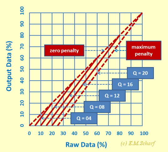
Fig. 7.1.2: Graphical Comparison of Raw Data and Averaging Marking Schemes
The graph in figure 7.1.3 is derived from the graph in figure 7.1.2 above, and shows the differences in the percentage output mark (K) (obtained by reading in the vertical direction) between the zero-penalty approach and intermediate penalty approaches where the number Q of questions attempted is 4, 8, 12, and 16 respectively, with the limiting case of Q = T = 20 being equivalent to the maximum penalty approach. For Q values of 4, 8, 12, 16 and 20, the corresponding maximum differences are thus 5, 10, 15, 20 and 25% respectively. Since the maximum difference can be as much as 25%, figure 7.1.3 emphasises that the mark that a student obtains for a MCT is strongly influenced by the way in which the educator processes the raw marks generated by the MCT.
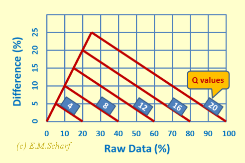
Fig. 7.1.3: Difference between Raw Data and Averaging Marking Schemes
7.2 Does a student benefit by guessing?
If there is no processing of the marks, in other words only the raw data are used as described in section 4, the answer is definitely yes for "blind" guessing. However, with the averaging approach of section 5, the answer is no. This is borne out by equation [5] and the table in figure 7.1.1. If Q, the total number of questions attempted, increases, but R, the actual score, stays the same, then the mark K actually given to the student will decrease. This is emphasised by figure 7.2.1. This shows the number of questions attempted against the resultant mark K for different raw scores (R) where R is the number of questions answered correctly, irrespective of whether this is due to the student's actual knowledge or to guessing. (Of course, in figure 7.2.1 we could also put odd values for R, but perhaps the message is put across to you the reader in a better way with a less complicated graph.) In figure 7.2.1, the downward sloping lines for given values of R indicate diminishing returns for the student if wrong answers, denoted by (Q-R), are given for further questions attempted.
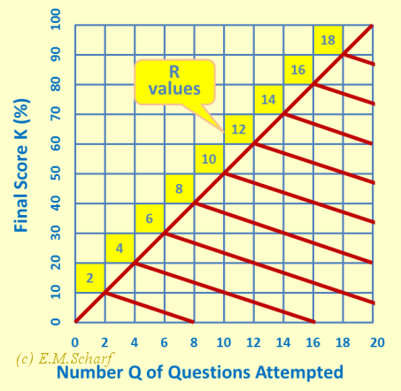
Fig. 7.2.1: Number (Q) of Questions Attempted against Final Score (K) for different numbers (R) of questions for which the correct answer is given (either from knowledge or by chance).
The effect of partial knowledge is also interesting. Suppose a student has additional partial knowledge that improves the chances of an answer being correct from 1/A to 1/P (i.e., P < A). For example, a student may be able to narrow down his or her options from 1 in 4 choices (A = 4) to 1 in 2 choices (P = 2). In this case, in equation [5], the subtracted term ((Q-R)/(A-1)) will be less in value if A is replaced by P where P < A. With partial knowledge, the negative impact on the final mark will, on average, be lessened. Naturally, this is only a very crude model of the situation since students will not normally approach each question with the same degree of partial knowledge.
7.3 Does the effect of guessing depend on A?
Does the effect of guessing depend on the number (A) of possible choices per question? Intuitively we could say that the more choices per question, the less the chance that a student hits on the right answer by blind guessing. In fact, we can say that the effect of guessing is proportional to (1/A), so that as A increases, the possibility of a student picking the right answer for a given question from a set of A possible answers diminishes. If we plot the probability as a percentage (instead of as a per unit) we get the graph shown in figure 7.3.1.
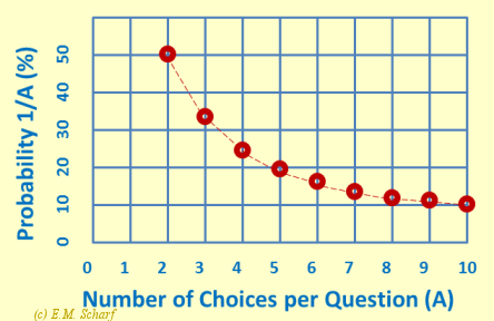
| A | 2 | 3 | 4 | 5 | 6 | 7 | 8 | 9 | 10 |
| probability 1/A (%) | 50.0 | 33.3 | 25.0 | 20.0 | 16.7 | 14.3 | 12.5 | 11.1 | 10.0 |
We have thus quantified our original statement that "the more choices per question, the less is the chance that a student hits on the right answer by blind guessing". Not only that, but figure 7.3.1 also shows us quantitatively that increasing the number of choices per question "indefinitely" is likely to bring the examiner diminishing returns when it comes to insuring against blind guessing by the student.
This and the next paragraph of the present section 7.3 are not required for an understanding of the material to be developed in later sections. However, as an exercise in manipulating the knowledge we have already gained in previous sections, we can also relate quantitatively the effect of guessing to an equation which we have indeed already established. We realize that figure 7.1.2 has been created by assuming for each question, four choices (i.e., A = 4), one of which is correct. In this figure we can see that the maximum difference DMAX in marks between the zero and maximum penalty lines is given by the vertical distance between the two lines from the crossing of the x-axis by the maximum penalty line; this distance is 25%. This exercise can be repeated by replotting figure 7.1.2 for different values of A, (e.g., A = 2 to A = 10).
|
[10] |
We short cut this effort of replotting several times, by considering equation [8]. For this equation we assume zero knowledge on the part of the student by putting KM = 0, despite the fact that the number of "right" answers is R = DMAX. This gives us a new equation [10] just above; using it, we can then dutifully plot and tabulate the results. This also gives us the graph shown in figure 7.1.3 above, except that now the y-axis would be labelled "Maximum Mark Difference", but otherwise the resultant graph and the units for its axes are identical.
7.4 Educator's Effort and the Number of Choices per question?
What is the optimum number (A) of choices for each question? Frequently, 3 or 4 choices are used. The greater the number (A) of choices, the more time must be allocated to a student to complete a question, but the smaller will be the influence of blind guessing by the student. From the teacher's perspective, the effort involved in providing a large number of choices per question means more time spent on assessment at the expense of contact time with the students.
Consider the following weighted cost function F(A), for which the term (αA) indicates the time spent preparing the question, where "α" is a weighting factor, and the term (β/A) indicates the effect of guessing, where "β" is a further weighting factor.
| DEFINITION |
|
[11] |
If we assume that all variables in equation [11] are positive, then equation [11] has a minimum for:
| key derived equation |
|
[12] |
If we look at the question in reverse and assume 3 or 4 choices per question, then equation [12] of course gives us an infinite number of corresponding matching ratios (β : α). The lowest values of the terms in the corresponding ratios are 9:1 and 16:1. In practical terms, this means that minimising the effect of guessing is regarded as being 9 or 16 times more important than the initial work in preparing the question. This fits in with normal practice. The emphasis on "initial work" highlights one advantage for the teacher of building up and maintaining a sizeable bank of multiple-choice questions. Of course, as has already been mentioned, another advantage of such a question bank, is to ensure the effect of novelty in the questions for the student.
7.5 Choices per Question and the Usable Range of Raw Marks
If we compare raw data and averaging approaches to processing MCT marks with two different values for A, the number of choices per question, and we then plot the results as in figure 7.5.2, we notice the following. While the gradients of the set of plots for a given value of A are identical, the gradients for different values of A appear to increase with increase in A. Thus, for A = 2, the gradient is arc tan (1) = π/4 radians or 45 degrees, and for A = 4, these values are steeper at arc tan (4/3) or 53.1 degrees. If A tends to infinity the angle would tend to 90 degrees.
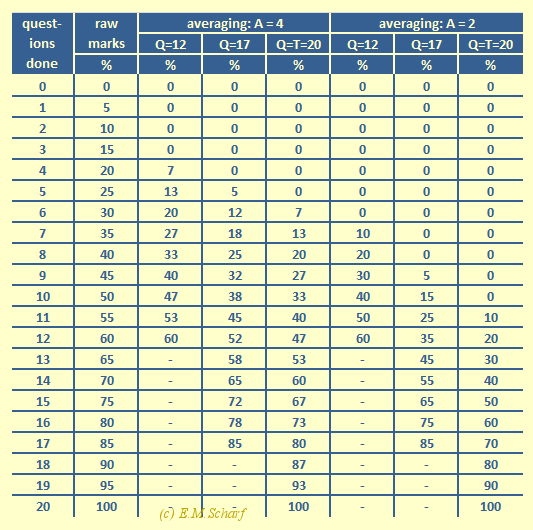
Fig. 7.5.1: Comparing raw data and averaging approaches to processing MCT marks with two different values for A, the number of choices per question.
The above figure (7.5.1) indicates that a larger value of A (the number of choices per question) gives a greater range of positive values in the results.
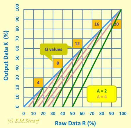
Fig. 7.5.2: Comparing raw data and averaging approaches to processing MCT marks with two different values for A, the number of choices per question. Plot of table in figure 7.5.1 above.
The steeper (i.e., larger) the gradient, the smaller the range of possible marks for a given value of Q. This is not desirable, but nor is the legitimate effort of producing too high a number A of choices per question. Somewhere there should be an "optimum" value of A, given these apparently conflicting aspects. To try and tackle this, we use equation [5] to establish the gradient which is then given by equation [13].
| key derived equation |
|
[13] |
This enables us to calculate, for a given value of A, the inverse gradient, expressed as a percentage - where we assume a maximum possible mark of 100%. So, for A = 4 we get 75% and for A = 2 we get 50%, both of which accord with the plots in figure 7.5.2. Where the maximum number of questions attempted is less than the number offered, we get a pro rata reduction in the maximum possible range of raw data marks. This also accords with figure 7.5.2. Thus, if we increase A, we increase the sensitivity of the processing of the marks to the available raw data marks. This is amplified in the table in figure 7.5.3 below. Of course, as we try and increase A indefinitely, we get diminishing returns regarding range sensitivity. In fact, as A tends to infinity, the plot in figure 7.5.2 indicates that the characteristic would tend to the characteristic (blue line) for the raw data approach, with of course, the added advantage of introducing the averaging approach.
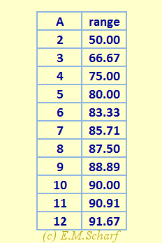
Fig. 7.5.3: Relative ranges for raw data (R) values for different numbers A of choices per question.
To clarify the concept of ranges we can also use the diagram of figure 7.5.4 below, which highlights ranges associated (for example) with Q = 12 (i.e., 12 questions attempted), and the corresponding available (usable) ranges R4 and R2 of raw data. From this it can be seen that the ratios R4/R∞ and R2/R∞ give 0.75 and 0.50 respectively as per the above table in figure 7.5.3.
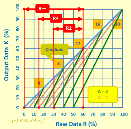
Fig. 7.5.4: Relative ranges R∞, R2 and R4 for raw data (R) values for Q = 12, and choices per question given by A = 2 and A = 4.
7.6 The Raw Data Line is the Limiting Case as A tends to Infinity
The Raw Data line (the blue diagonal line) in figures 7.5.2 and 7.5.4 can be regarded as the limiting case, as A tends to infinity, of both the raw data and the averaging methods.
- Averaging. In equation [5], as A tends to infinity, K tends to R - i.e., the number of questions, R, answered in the right way, tends to the number K of questions whose respective answers are known. Thus, in figures 7.5.2 and 7.5.4, the "Raw Data" line (the blue diagonal line) in the limiting case of the green and purple lines (for A = 4 and A = 2 respectively for Q = 20 (i.e., all questions attempted). For Q less than 20, the corresponding smaller lines for A = 2 and A = 4, will tend to a corresponding smaller raw data line as A tends to infinity.
- Raw Data. In section 6.2 we remarked that the zero penalty (raw data) option is not ideally suited to an examination context, since it will, on average, give a student Q/A marks - even if that student has no knowledge whatsoever of the exam subject. However, as A tends to infinity, it can be seen that also in the "raw data" or zero penalty case, K tends to R.
7.7 Distribution of Marks for Each of Our Three Approaches
Here we provide a further insight into the distinction between the the three approaches (1) raw data, (2) averaging, which uses number of questions attempted, and (3) maximum penalty, which uses number of questions offered. We take the case where A = 4 and T = Qmax = 20.
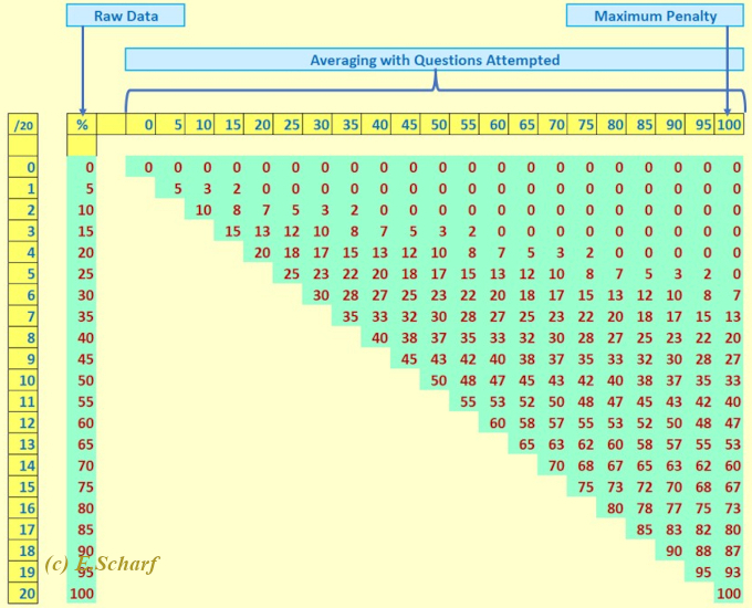
Fig. 7.7.1: Relative ranges of (a) raw data, (b) averaging with questions attempted, and (3) maximum penalty approaches. Here, A = 4 and T = Qmax = 20.
From figure 7.7.1 above, we can draw the following inferences.
- Raw Data. On the left we have the vertical "raw data" column. This contains the possible results with this approach. However, as we know, anyone, even if they know nothing about the subject being examined, can, with A=4, on average, obtain 25% of the available marks for the exam.
- Maximum Penalty. On the right, we have the vertical "maximum penalty" column. With this approach, questions which are not even attempted are treated as having the wrong answer. For A=4, the first six possible results are all zero. The range of possible marks is restricted to 7% to 100%
- Averaging. With the "averaging approach" we have twenty-one (20 + 1) possible vertical columns covering results across the spectrum from 0% to 100%. Each vertical column represents the maximum number of questions attempted by a candidate (one or more), as opposed to the number of questions offered to all candidates. Essentially we do not waste "results space". The possible marks for a class - for a class test - are thus spread out across the full range of marks. For each exam participant (indicated by one of the twenty-one (20 + 1) vertical columns), apart from the maximum 5% case, there are 6 or 7 marks between successive possible marks - indicating an even spread. Note also our earlier comment about the number of wrong answers influencing a given candidate's result.
8. Subtractive Strategy
The subtractive approach is generally "harsher" than the "averaging" approach. Like the latter, the subtractive approach can also use either the number of attempted questions or the number of offered questions. Here we shall look at the following aspects.
- What is the Subtractive Approach?
- Subtractive - using questions offered
- Numerical Comparisons between Averaging & Subtractive Approaches
- Critique of the Subtractive Approach
8.1. What is the Subtractive Approach?
In this strategy, right answers will cause marks to be added into the total of questions; for every "non-right" answer we subtract 1 or more. Subtraction is typically done to penalize (discourage) guessing. As before, in sections 5 and 6, R represents the raw marks; Q represents the number of questions attempted. The number (Q-R) of "non-right" answers is multiplied by a factor we shall call G.
This gives equation [14]. Here, to avoid confusion, J is used now instead of K to represent the number of questions whose answers are, according to the "subtractive" method, regarded as known. Thus, a right answer will contribute 1 to J. A "non-right" answer could cause 1 or more to be subtracted from J, depending on the value specified for G. In the present subtractive case, it is not good enough for a student to know the answer to a question; there is additional pressure for a student not to give a wrong answer.
G could typically be one, but could more generally be a factor other than one, e.g., 0.5, 1.5 or 2. If G is zero, we have the "raw data" situation, with no processing.
| DEFINITION |
|
[14] |
Let us use the following substitution for G.
| DEFINITION |
|
[15] |
This gives us equation [16], which is algebraically equivalent to equation [5]. However, for "subtractive" processing, A and K in equation [5] are replaced by B and J respectively, in order to estimate the numbers of questions actually known.
|
[16] |
This yields a mathematically convenient formulation - convenient in that it is similar to the previous formulations using A. For G = 1, 1/2, 1/3, we have equivalent values B = 2, 3, 4 respectively. However, it should be emphasized and reiterated that for the subtractive processing strategy, G (and by implication B) is actually independent of, and chosen separately from, the actual number A of choices per question. The means that in the subtractive case, as outlined here, we are not directly taking account of the number, A, of choices per question. Remember that it is A that allows us to control the influence of guessing without using an overtly unpopular penalizing approch anchored in G (i.e. B).
8.2. Subtractive - using questions offered
A variation of this strategy is to put Q=T, as in section 6.4. In other words, we also regard questions that have not been attempted as wrongly answered questions (i.e. as having been given "non-right" answers by the candidate). In this case we replace Q by T. Equation [15] relating G to B is of course still valid, and so is the fact that for this marking strategy, G is independent of the actual number A of choices per question.
8.3. Numerical Comparisons between Averaging & Subtractive Approaches
Here you will see figures 8.3.1 and 8.3.2, which are essentially the same as figures 7.5.1 and 7.5.2, but with A = 2 replaced by G = 1. G = 1 is a popular value when applying the subtractive method of processing MCT marks. Essentially, for every wrong answer we subtract one mark from the final total, where, as we said, each correct answer carries one mark.
Let us try to clarify a bit further as to what we are doing here.
- For the averaging case below we are using 4 choices per question (i.e., A = 4); we also use A to modify the raw data R according to equation [5] above.
- For the subtractive case below, we still use A=4 for the number of choices, but modify the raw data R according to equation [16] above, in which J now represents our estimate of the number of questions whose answers the student actually knows.
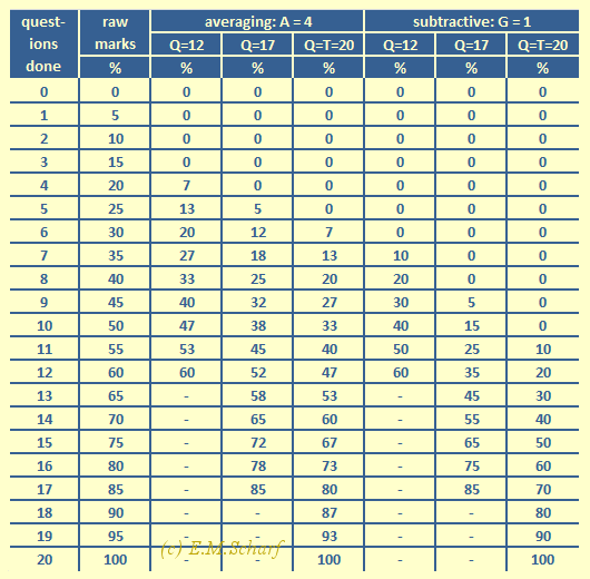
Fig. 8.3.1: Comparing raw data, averaging and subtractive approaches to processing MCT marks.
With both averaging and subtractive approaches, non-zero marks start later than when using with the raw data approach. This effect is more noticeable with the subtractive approach.
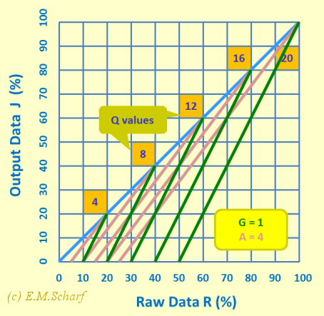
Fig. 8.3.2: Comparing raw data and averaging approaches to processing MCT marks with A = 4 and G = 1. Plot of table in figure 8.3.1 above.
In figures 8.3.1 and 8.3.2, it is assumed that we consider the number Q of questions attempted and only the total number of questions offered in the limiting case of Q = 20 (or 100% when scaled). In these figures you can thus see, that the slopes for G = 1 are steeper than those for the average MCT processing method using the popular choice of A = 4. The marking for the subtractive approach is noticeably more sensitive with change in the raw data R values than for the averaging approach. Put another way, to achieve the same output mark (K or J), a greater range of raw data marks is required in the averaging approach (chapter 6) than in the subtractive approach - which many would see as an aspect favouring the averaging approach (chapter 6).
The table in figure 8.3.3 is constructed in the manner of the table in figure 7.5.3 and serves to amplify the way that the range of available raw data values deteriorates as G increases. As before, the maximum available range should be reduced pro rata according to the maximum number of questions actually attempted.
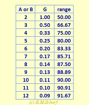
Fig. 8.3.3: Relative ranges for raw data (R) values for different G values.
8.4. Critique of the Subtractive Approach
We could, of course, introduce two stages to the processing of the raw data R. We could (1) first estimate K using the averaging approach, and (2) then use the subtractive approach to further reduce K. This could penalize the student massively, apart from making the processing of the raw data R more complicated, thereby increasing the chance for errors in the manual or software processes that we use, and also potentially introducing additional rounding errors when producing the final integer mark. Another option with the Subtractive Scheme could be to reward "right" answers by (e.g.) adding 2 instead of 1 to the marks total. The rationale for these options would potentially need to be justified to an external examiner at a college examination board. The question might be, "How does the particular processing structure (reward and penalty), chosen for use with the subtractive approach, actually help to assess a candidate's knowledge?"!!!
The maths associated with the Subtractive Scheme are shared with those of the Averaging Scheme. However, as just mentioned, the rationale for the "B" value of the subtractive scheme is likely to be more difficult to justify to an external examiner at a college examination board, than the rationale for the "A" value of the averaging scheme, where of course, the "A" value represents the number of choices per question and can also be used in a statistical model, however basic that model may be.
To emphasize, we have an important distinction between averaging and subtractive approaches.
- Averaging. The mathematics associated with the averaging approach are clearly associated with the structure of the questions. This provides consistency between different MCTs conducted by a teacher. With the averaging approach, R (number of "right" questions) and K (number of questions for which the answer is known) are explicitly linked.
- Subtractive. The choice of the value for "B" and the choice of the number of marks to be added or subtracted for a question, do not provide a clear link between R and K.
9. Future Challenges
Multiple-choice tests have gained great popularity with students, especially when the tests are computer-based, and with teachers who, by saving on assessment time, can devote more resources to the actual process of teaching. However, the following possibilities show that there are still many challenges with setting and devising MCTs.
- Statistical Assumptions.
The averaging assumption is of course just one of a vast variety of statistical assumptions that could be employed. For example, in formulating assumptions leading to a suitable model, the following questions could also be considered.
- Does the averaging process reflect the true statistics associated with a student's thought processes?
- Could the statistics also be influenced, for example, by the way the particular course (whose students are being examined by the MCT), is actually taught and delivered to the student?
- Reassuring the Student.
Examples in this area include good interfaces and possibly adjusting the marking scheme.
- Good Interfaces. A good computer interface can encourage and put students at their ease. A good layout of a printed version of an MCT can also be beneficial to the student.
- Adjusting Marking Scheme. There are many possibilities. A basic one is to consider a compromise between the no-penalty option 1, which encourages students to supply answers and option 2 which discourages guessing could be used. This might be achieved, when processing the raw marks, by making the factor "A" more than the number of available question choices.
- Revealing Thinking Patterns. This is a fundamental consideration. Basic MCTs only test factual knowledge, but by careful attention to the question, thinking processes could be deduced. Marks could then be allocated not only on the basis of whether the question was correctly or incorrectly answered, but also on how the student reached his or her conclusion. More work is needed here to formalise the process. Work on Item Response Theory [ref6] moves in this direction. Interesting work (e.g. [ref7], [ref8] and [ref9]) has been also conducted in areas where the task given to the student is tightly constrained, such as producing a computer program.
10. Conclusions
We should remember that in the first instance, the computer conveniently gathers the raw marks for us; what we do - or ask the computer subsequently to do - with those marks is up to us as the assessors and could have a significant impact on a student's marks in the MCT.
Whilst multiple-choice tests (MCTs) readily lend themselves to automatic marking, we can see that one of the challenges of MCTs lies in the need - since we do not know the number C of questions got right by chance - to make some sort of assumption, to enable us to use the MCT to assess what a student actually knows. The averaging assumption given by equation [3] is certainly usable, especially where no other factors such as a student's partial knowledge, the way that a course has been taught or errors due to some distraction are, or can be, assumed.
|
In many cases it may not be enough to say that a student has got the right answer to a multiple-choice question. We would wish to ask whether or not the student actually knows the answer to the question. |
A number of marking schemes for MCTs have been considered on this web page. The following table (fig. 10.1) aims to relate these schemes to their predominant features.
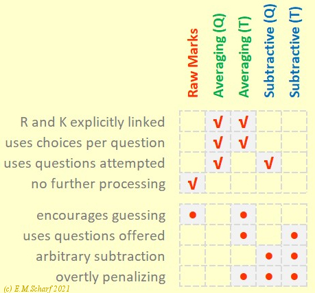
Fig. 10.1: Summarizing raw data, averaging and subtractive approaches to processing MCT marks.
(Q) and (T) indicate questions attempted and offered respectively.
The first four features (☑) are seen as advantages.
Raw Data? Using the averaging assumption of equation [3], we have suggested that the raw data marking scheme is unfair to the marker or examiner, and indeed ultimately to the student, in that students can get marks by blind guessing, without knowing anything about the subject at all.
Subtractive Approach? The subtractive approach is unfair to the student in that it overly restricts the range of possible raw data marks that could actually produce output marks for the student. The maths associated with the Subtractive Scheme are shared with those of the Averaging Scheme. However, the rationale for the "B" value of the subtractive scheme is likely to be more difficult to justify to an external examiner at a college examination board, than the rationale for the "A" value of the averaging scheme - where of course, the "A" value represents the number of choices per question and can also be used in a statistical model, however basic that model may be.
Averaging Approach? It is suggested that the fairest approach is the averaging approach, where a selection of A = 4 for the number of choices per question provides a balance between (1) the range of raw data marks attracting processed marks, (2) a reasonable hedge against the effect of guessing by the student and (3) not too great a need to introduce fake or dummy choices for each question.
Questions Offered or Attempted? Another recommendation is to consider the number of questions attempted as opposed to the total number of questions offered, should on any occasion the latter exceed the former. By considering the number of questions actually attempted, we ensure that the results are based on a student's actual efforts in the exam, in the manner of a conventional written paper. This is helped if, in the MCT exam, a student is able not just to change, but also to cancel completely, the answer he or she has given to any given question.
|
ADVANTAGES FOR THE
QUESTION-SETTER (EXAMINER) Using the Averaging Approach together with the questions actually attempted offers the following advantages over the use of raw data and over the use of the maximum penalty approach.
The Averaging Approach offers the following advantage over the use of the Subtractive Approaches.
|
11. References & Links
While the amount of literature on multiple-choice tests is quite extensive, there appears to be little in the way of a discussion on how to process and evaluate the marks arising from such tests, marks which are often collected automatically and at great speed. Possibly a question, by the setters of MCTs, of acting in haste and repenting at leisure! However, the first set of the following references is directly relevant to the aims of this web paper, the second set is tangentially relevant.
11.1 Main References
| [1] |
Eric M. Scharf and Lynne Baldwin,
Assessing multiple-choice question (MCQ) tests - a mathematical
perspective,
Active Learning in Higher Education,
Sage Publications,
DOI: 10.1177/1469787407074009,
Vol 8(1): pages 33-49, 2007. Available at: http://alh.sagepub.com/cgi/content/abstract/8/1/31 (This paper contains a number of relevant references). |
|
| [3] |
Robert B. Frary,
Formula Scoring of Multiple-Choice Tests (Correction for Guessing) -
Teaching Aid, Educational Measurement: Issues and Practice,
National Council on Measurement in Education, 1988, 7(2), http://ncme.org/publications/items/, accessed: 2012-12-12. |
|
| [4] |
Australian Mathematics Trust,
AMC Scoring System,
Australian Mathematics Trust, http://www.amt.edu.au/amcscore.html, accessed: 2013-01-08. |
|
11.2 Further References
| [6] |
Frank Baker,
Item_response_theory, December 2001 http://echo.edres.org:8080/irt/, accessed: 2012-12-12. |
|
| [7] |
Michael J. Rees,
Automatic assessment aids for Pascal programs, Newsletter, ACM SIGPLAN Notices, Volume 17 Issue 10, October 1982 Pages 33 - 42, ACM New York, NY, USA, DOI: 10.1145/948086.948088, http://dl.acm.org/citation.cfm?id=948088, accessed: 2012-12-12. |
|
| [8] |
David Jackson,
A software system for grading student computer
programs,
Computers & Education, Volume 27, Issues 3-4, December 1996,
Pages 171-180. http://www.sciencedirect.com/science/article/pii/S0360131596000255, accessed: 2012-12-12. |
|
| [9] |
Riku Saikkonen, Lauri Malmi, Ari Korhonen,
Fully automatic assessment of programming
exercises,
ITiCSE '01 Proceedings of the 6th annual conference on Innovation and
technology in computer science education,
Volume 33 Issue 3, Sept. 2001, Pages 133-136, ACM New York, NY, USA -2001,
ISBN:1-58113-330-8,
DOI: 10.1145/377435.377666. http://dl.acm.org/citation.cfm?doid=377435.377666, accessed: 2012-12-12. |
12. Symbols and Abbreviations
To keep life simple, only important symbols and those that are not local to a particular section are included here. This section therefore serves an aide-memoire to try and make the life of you the reader as straight forward as possible when negotiating some of the more - sometimes inevitably intertwined - sections of this web paper.
12.1. Symbols
In the table below, symbols are grouped according to the section (§) in which they first occur. Please also remember that, in furtherance of simplicity, we have assumed, without loss of generality, one mark per question. This means, for example, that the number of raw marks (marks for right answers) translates directly and without scaling to the actual raw marks themselves.
|
| | | | | | | | | |
|
12.2. Abbreviations
| MCQ | Multiple-Choice Question | |
| MCT | Multiple-Choice Test |
Appendix
13. Finding the Number Q of Questions Attempted
We are suggesting in this web paper that using Q, the number of questions attempted, can be fairer to the student than using T, the number of questions offered. This indeed is the message from the section 7.1, above. Hence, the following should be available to the examiner.
- Scripts. Hard Copy OR Digital
- Hard Copy Scripts. From hard copy exam scripts, the number Q of questions attempted should be evident for each candidate.
- Exam Output in Digital Form. From exam output created by an on-line MCT utility, the number Q of questions attempted by each candidate should be made available to the examiner.
- Cancellation Facility. If the candidates are able to cancel the answer to any question, it should be possible for Q to be modified/updated as a result.
Latest Update: 2023-10-05 @11:27
Please Refresh Page for Latest Version!
SAGAX REX HANC RETIS ORBIS PAGINAM PINXIT
ANNO MMXI ET MMXVII ET MMXX ET MMXXI ET MMXXII ET MMXXIII
© Eric Scharf 2011 & 2017 & 2020-2023